Why was attention needed?

The performant architecture of the day circa 2014 were RNNs. They performed remarkably well on tasks like machine translation compared to prior model types. However, they suffered from 2 main disadvantages:

1. Long range dependencies: Theoretically, the current hidden state of an RNN contains information relating to all previous states due to its recurrent nature. However, practically training these networks with backprop leads to the vanishing or exploding gradient problem since contribution of an early time step can propogate signal that arbitrarily large or small as it passes through the layers. LSTMs and GRUs introduced gating mechanisms to deal with these dependency issues, but struggled with very long sequences as well.
2. Lack of parallelism: In RNNs, the prior tokens needed to be processed in order for the next token to be processed due to the nature of the architecture. This approach left a lot on the table in terms of taking advantage of the massive parallelism enabled by advances in GPU hardware, which were the devices on which neural networks and tensor ops took place on. In contrast, modern transformer architectures enable each token to interact with every other token in the sequence simulataneously - allowing for much faster training of models.

Attention was initially invented to augment RNN models, so that the model can focus on different parts of the input sequence as the output sequence is being generated.

What is attention?

The core analogy of attention comes from classic information retrieval system -

1. Query (Q) represents what a specific token in the input is “looking for” in the sequence.
2. Key (K) represents what each token “offers” and how it can be identified by others.
3. Value (V) represents the actual content or information in a specific token.

To note, in self-attention the Q, K and V vectors are all derived from the same source, typically the output of the previous layer. This allows each to token to dynamically compute attention scores against each token in the sequence (including itself, effectively teaching itself which tokens are important to understand its own meeting within its context).

Setup

Attention mechanisms form the backbone of the transformer architecture, powering the latest variant of LLMs near you. Here, we will delve into core concepts of attention, build towards the transformer architecture and then review some efficient attention modifications including some hardware-aware optimizations.

Before we dive into attention, let’s establish our inputs we will be playing around with.

Code: Setup

 1
 2
 3
 4
 5
 6
 7
 8
 9
10
11
12

# Pre-reqs - basic pytorch knowledge

import torch
import torch.nn as nn
import torch.nn.functional as F
import math

# Imagine we have a batch of sequences, and each token is represented by an embedding.
batch_size = 2
seq_len = 3 # e.g. The, synapse, conducts
embed_dim = 4 # This is often called d_model in papers, e.g. 768 in BERT
input_embeddings = torch.randn(batch_size, seq_len, embed_dim)

We have a 3 token toy example, which is projected into an embedding dimension of size 4.

Core concepts

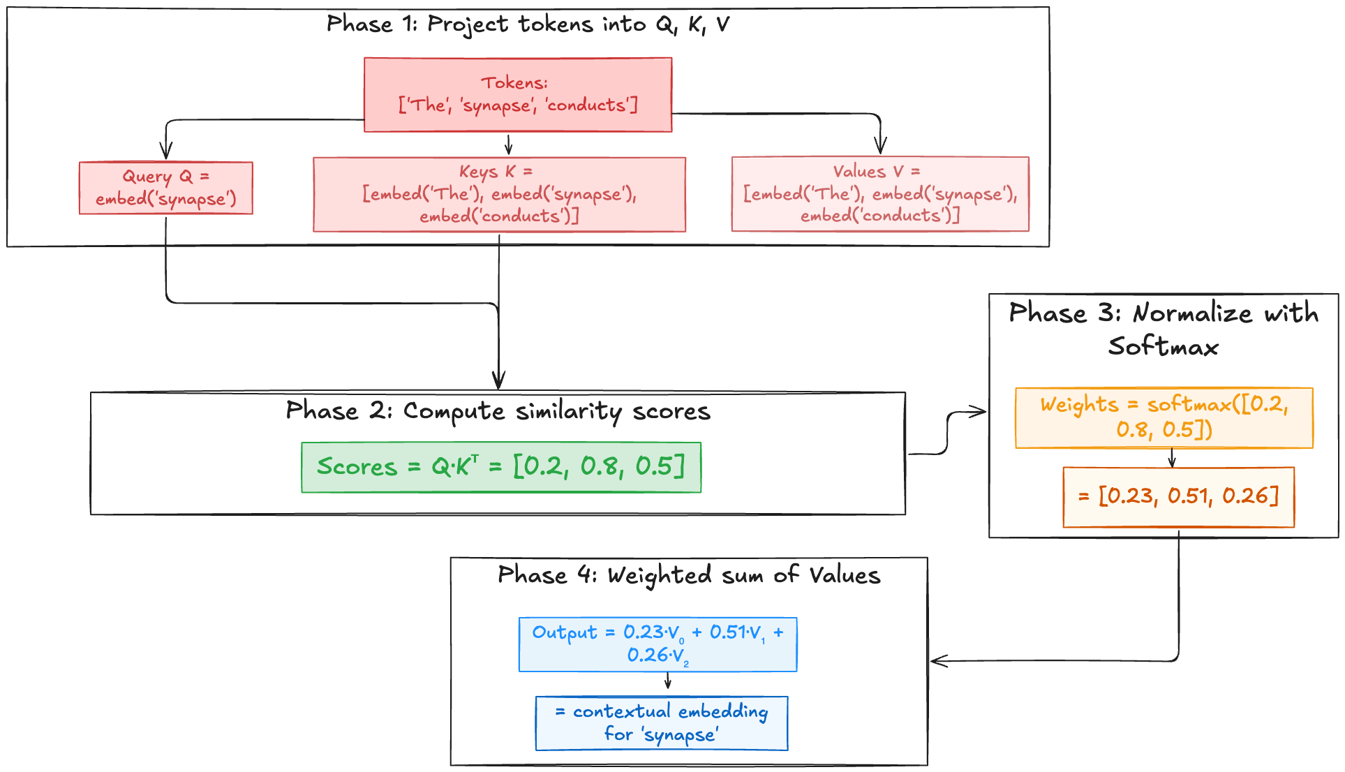
This QKV setup is like a “soft” dictionary lookup. In a regular dictionary, you provide an exact query (a word), find its matching key, and retrieve the value (the definition). In attention, the query doesn’t need to be an exact match. Instead, it finds how similar or relevant each key is, and then retrieves a blend of values based on these relevance scores.

Crucially, Q, K, and V are not typically the raw input embeddings themselves. They are usually obtained by applying separate learned linear transformations (weight matrices \( W_Q \), \( W_K \), \( W_V \)) to the input embeddings.

where \( X \) is the matrix of input embeddings.

In code, we’ll use linear layers to do these matrix projections.

Note: the dimensions of \( Q \), \( K \), \( V \) can be same or different. For simplicity now, let’s keep them as embed_dim, but especially in multi-head attention, d_k (dim of \( K \)) often equals d_v, and d_q can also be the same, often set to d_model/num_heads.

Code: QKV computation

 1
 2
 3
 4
 5
 6
 7
 8
 9
10
11
12
13
14
15
16
17

# input_embeddings from Setup = X

d_q = d_k = d_v = embed_dim # For simplicity in this initial example

W_q = nn.Linear(embed_dim, d_q, bias=False) # bias=False is common in Transformer QKV projections
W_k = nn.Linear(embed_dim, d_k, bias=False)
W_v = nn.Linear(embed_dim, d_v, bias=False)

# Let's generate our Q, K, V matrices
Q = W_q(input_embeddings)  # X.W_q - Shape: (batch_size, seq_len, d_q)
K = W_k(input_embeddings)  # X.W_k - Shape: (batch_size, seq_len, d_k)
V = W_v(input_embeddings)  # X.W_v - Shape: (batch_size, seq_len, d_v)

print(f"Input Embeddings shape: {input_embeddings.shape}")
print(f"Q shape: {Q.shape}")
print(f"K shape: {K.shape}")
print(f"V shape: {V.shape}")

\( W_Q \), \( W_K \), \( W_V \) are learnable weight matrices or model parameters. They allow the model to learn different projections, and this is what allows the model to focus on different aspects of the input for different roles in the attention mechanism. This makes the system very flexible and robust to different inputs and scenarios!

Scaled Dot-Product Attention

The dominant attention mechanism used in Transformers and many other modern architectures is Scaled Dot-Product Attention.

The formula is:

where:

• \( Q \) is the matrix of queries
• \( K \) is the matrix of keys
• \( V \) is the matrix of values
• \( d_k \) is the dimension of the keys (used for scaling)

These projections should start looking familiar now -

1. Compute dot products (similarity scores; phase 2):

   $$ Scores=QK^T $$

   It always helps in matrix math to imagine the dimensions - if \( Q \) has dimensions \( (N_q, d_k) \) (number of queries, dimension of queries=keys) and \( K^T \) has dimensions \( (d_k, N_k) \) (dimension of queries=keys, number of keys), the resulting \( Scores \) matrix will have dimensions \( (N_q, N_k) \). Each element \( Scores_{ij} \) represents the similarity between the \( i \)-th query and the \( j \)-th key.

2. Scale:

   $$ \text{ScaledScores} = \frac{Scores}{\sqrt{d_k}} $$

Role of scaling factor

The dot-product of query (Q) and the transpose of key (K^T), when the dimensions of the key vector (d_k) grow large in magnitude. When we pass these into the softmax function, they can push the function into regions where its gradients are extremely small, effectively halting the learning process or making it unstable. Hence, scaling this dot-product by a factor (d_k) counteracts this by bringing the gradients to a more stable range, and preventing the saturation of the softmax.

As \( d_k \) increases, it linearly increases the variance of the \( Q.K \) dot product, which when fed into the softmax, makes the scaled scores very sparse (weighing heavily towards the highest value). Let’s understand more intuitively.

The softmax formula is:

Let the key/query dimension be \(d_k = 4\).
We have one query vector

And two key vectors

if we compute unscaled dot-product scores

Softmax without scaling -

Even here, the distribution is already quite “peaky”. For larger \(d_k\), raw dot-products can be much bigger, making softmax even more extreme (e.g. one value ≈ 0.99, the other ≈ 0.01).

If we apply scaling, Since \(\sqrt{d_k} = \sqrt{4} = 2\), we divide each score by 2:

Softmax with scaling -

The distribution is less extreme (0.73/0.27 vs. 0.88/0.12), which:

• Keeps gradients larger for the “losing” key (\(K_2\)), aiding learning.
• Prevents softmax saturation when \(d_k\) (and thus raw dot scores) grows.

3. Apply softmax:

This normalizes the scores into a probability distribution, where attention weights sum to 1.

4. Weighted sum of values: Finally, we multiply the attention weights by the value matrix \( V \) to get the output of the scaled dot product attention layer.

If \(\text{AttentionWeights}\) has dimensions \((N_q, N_k)\) and \(V\) has dimensions \((N_k, d_v)\) (number of keys, dimension of values), the \(Output\) will have dimensions \((N_q, d_v)\). Each row of the output is a weighted sum of the value vectors, where the weights are determined by how much each key (corresponding to a value) matched the query.

Masking

Masking is used in practice to prevent attention to certain positions. They are usually:

• Padding masks in batched processing: Sequences of different lengths are often padded to the same length. We don’t want the model to pay attention to these padded tokens. A padding mask if applied, which sets the attention scores for these positions to a very large negative number (neg. infinity) before the softmax step. This ensures that their contribution to the softmax probability is effectively zero.
• Causal masks: Look-ahead masks for auto-regressive tasks like language generation in a decoder, a token at a given position should only attend to the previous tokens and itself, and not to future positions. A causal mask sets these future tokens to neg. infinity.

In practice, PyTorch’s torch.nn.functional.scaled_dot_product_attention function provides an optimized implementation, handling scaling and masking internally. It also has optimizations like FlashAttention built-in.

Code: Scaled Dot-Product Attention

 1
 2
 3
 4
 5
 6
 7
 8
 9
10
11
12
13
14
15
16
17
18
19
20
21
22
23
24
25
26
27

# Step 1: Calculate Q.K_T
K_T = K.transpose(-2, -1) # (batch_size, seq_len, d_k) -> (batch_size, d_k, seq_len)
scores = torch.matmul(Q, K_T)

# Step 2: Scale
# d_k is the dimension of the key vectors, which is K.size(-1)
scale_factor = math.sqrt(K.size(-1))
scaled_scores = scores / scale_factor

# Step 3: Apply softmax to get attention weights
attention_weights_scratch = F.softmax(scaled_scores, dim=-1)

# Step 4: Multiple weights by V to get the output
output_scratch = torch.matmul(attention_weights_scratch, V)

####################################

# Using torch.nn.functional.scaled_dot_product_attention
output_f, attention_weights_f = F.scaled_dot_product_attention(Q, K, V, attn_mask=None, dropout_p=0.0, is_causal=False, need_weights=True)

# is_causal = True will create a causal mask
# under the hood, it basically does this - creates a lower triangular mask so that a token only attends to itself and every token before it.
causal_attn_mask = torch.tril(torch.ones(seq_len_q, seq_len_k, dtype=torch.bool))
# .unsqueeze(0).unsqueeze(0) to match dims and pass as attn_mask

# You can apply similar logic for padding masks

Additive vs. Multiplicative/Dot-Product

Although transformer models have standardized the use of scaled dot-product attention, it is good to know that there have been other types of attention mechanisms that were used for models like RNNs.

Additive Attention (Bahdanau)

This mechanism, introduced by Bahdanau, computes attention scores using a small feed-forward network. The decoder’s current (or previous) hidden state and each encoder hidden state are concatenated and passed through a feedforward layer to produce a score. Because it uses vector addition and nonlinearity internally, it’s called additive attention.

The general formula for the alignment score \( e_{ij} \) between a decoder hidden state \( s_{i-1} \) (query) and an encoder hidden state \( h_j \) (key) is:

where \( W_a \), \( U_a \) are weight matrices, \( b_a \) is a bias term, and \( v_a \) is a weight vector. The \( \tanh \) function provides a non-linearity. The core idea is to project both \( s_{i-1} \) and \( h_j \) into a common hidden dimension, combine them (often through addition), apply a non-linearity, and then project this down to a scalar score. This approach allows the model to learn a potentially more complex, non-linear similarity measure between the query and key vectors.

Multiplicative (Luong/Dot-Product) Attention

Luong proposed a simpler, more computationally efficient attention mechanism, often called multiplicative or dot-product attention. Instead of using a feed-forward network, the alignment score is computed directly as a dot product (or a general linear transformation) between the decoder hidden state and the encoder hidden state.

The most common forms are:

• Dot:

  $$ \text{score}(s_i, h_j) = s_i^\top h_j $$

  (if dimensions match)

• General:

  $$ \text{score}(s_i, h_j) = s_i^\top W_a h_j $$

  (where \(W_a\) is a learnable weight matrix)

• Concat (similar to Bahdanau but often grouped here):

  $$ \text{score}(s_i, h_j) = v_a^\top \tanh(W_a [s_i; h_j]) $$

  (concatenate then project)

Scaled Dot-Product attention, as used in Transformers, is a specific and highly optimized form of multiplicative attention.

In summary, Bahdanau’s additive attention introduces extra parameters (learned weights in a small neural net) to compute alignment scores, potentially giving more flexibility at the cost of speed. Luong’s multiplicative (dot-product) attention relies in the representation power of the high-dimensional vectors to measure relevance via dot products. Empirically, dot-product attention is faster and easier to implement, while additive attention can be slightly better for very fine-grained alignment in some cases (though the difference is often small).

Transformers

Self-Attention

Self-attention is basically attention where the queries, keys and values originate from the same sequence (essentially what we have been doing so far). This process recalculates the representation of each token based on how its meaning is influenced by other tokens in the sequence, thereby creating context-aware embeddings.

For instance, in “I am sitting on a river bank”, self-attention would help the model understand that “bank” = “side of river” due to the presence of “river”. Conversely, in “I am sitting in a bank to withdraw money”, self-attention would associate “bank” with financial institutions due to words like “withdraw” and “money”.

An important thing to note is that self-attention is actually permutation invariant. This means that if the input sequence is shuffled, the self-attention output for each token would be the same weighted sum of value vectors, just potentially with permuted attention weights corresponding to the shuffled keys. The inherent relatedness score between any two tokens (derived from their Q and K vectors) doesn’t change if their absolute positions change but their content doesn’t. This is why we need positional encodings - they inject information about the token order into the embeddings, allowing self-attention to differentiate based on position as well as the content.

Let’s build the Self-Attention model in pytorch based on what we have done so far.

 1
 2
 3
 4
 5
 6
 7
 8
 9
10
11
12
13
14
15
16
17
18
19
20
21
22
23
24
25
26
27
28
29
30
31
32
33
34
35
36
37
38
39
40
41
42
43
44
45
46
47
48
49
50
51
52
53
54
55
56
57
58
59
60
61
62
63
64
65
66

class DotProductAttention(nn.Module):
    def __init__(self, dropout=0.0):
        super().__init__()
        # add dropout here if needed
        self.dropout = nn.Dropout(dropout)

    def forward(self, query, key, value, attn_mask=None, is_causal=False):
        # expected shape of Q,K,V - (batch, heads, seq_len, dim)
        # attn_mask: shape should be broadcastable to (batch, heads, seq_len_q, seq_len_k)
    
        d_k = query.size(-1)

        # Q.K_T gives the raw similarity
        # Scaled dot product attention formula
        scores = torch.matmul(query, key.transpose(-2, -1)) / math.sqrt(d_k)

        if is_causal:
          seq_len_q = query.size(-2)
          seq_len_k = key.size(-2)
          causal_mask_manual = torch.triu(torch.ones(seq_len_q, seq_len_k, dtype=torch.bool, diagonal=1))
          
          if scores.ndim == 4: # (batch, heads, seq_len_q, seq_len_k)
            causal_mask_manual = causal_mask_manual.unsqueeze(0).unsqueeze(0).expand(scores.size(0), scores.size(1), -1, -1)
          elif scores.ndim == 3: # (batch, seq_len_q, seq_len_k)
            causal_mask_manual = causal_mask_manual.unsqueeze(0).expand(scores.size(0), -1, -1)

          scores.masked_fill_(causal_mask_manual, -float("inf"))
        
        if attn_mask is not None:
          # elements of attn_mask = True -> mask these out
          scores.masked_fill_(attn_mask, -float("inf"))
        
        attention_weights = F.softmax(scores, dim=-1)
        attention_weights = self.dropout(attention_weights)
        output = torch.matmul(attention_weights, value)
        return output, attention_weights


class SelfAttentionModule(nn.Module):
  def __init__(self, embed_dim, d_qkv, dropout=0.0): # d_qkv is dimension after projection
    self.W_q = nn.Linear(embed_dim, d_qkv)
    self.W_k = nn.Linear(embed_dim, d_qkv)
    self.W_v = nn.Linear(embed_dim, d_qkv)
    self.attention = DotProductAttention(dropout)

  def forward(self, x, padding_mask=None, is_causal=False):
    Q = self.W_q(x) # (batch_size, seq_len, d_qkv)
    K = self.W_k(x)
    V = self.W_v(x)

    # padding_mask shape is (N, S_k) -> attn_mask (N, 1, S_k) -> broadcast to (N, S_q, S_k)
    attn_mask_expanded = None
    if padding_mask is not None:
      attn_mask_expanded = padding_mask.unsqueeze(1).expand(-1, x.size(1), -1) # broadcast to (N, S_q, S_k)
      # to use with F.scaled_dot_product_attention,
      # attn_mask_expanded = ~padding_mask.unsqueeze(1)
    output, attn_weights = self.attention(Q, K, V, attn_mask=attn_mask_expanded, is_causal=is_causal)
    

    # output = F.scaled_dot_product_attention(
    #     Q, K, V,
    #     attn_mask=attn_mask_expanded,
    #     dropout_p=self.dropout_p,
    #     is_causal=is_causal
    # ) - doesnt return attn_weights
    return output, attn_weights

Multi-Head Self-Attention (MHSA)

Multi-Head Self-Attention enhances self-attention by allowing the model to jointly attend to information from different “representation subspaces” at different positions. The intuition is that a single attention mechanism might average away or focus on only one type of relationship. By having multiple “heads,” the model can learn different types of relationships or focus on different aspects of the input simultaneously. For example, one head might focus on syntactic dependencies, another on semantic similarity, and yet another on co-occurrence patterns.

The idea extends to the all the steps of the self-attention mechanism.

Linear projections for \(Q, K, V\) - Instead of projecting to a 2D weight layer, we use a 3D weight layer \(W\) where each head gets its own 2D matrix \(W_i\). For each head, we will have,

Typically, we will have dimensions of \(d_q = d_k = d_v = d_head = d_\text{model}/h\), which means that the original embedding dimension of the model will be split among the heads. Alternatively, we could project a single large linear projection, and the reshape and split.

Now, we basically follow the steps of scaled dot product self-attention for each head in parallel and then concatenated in the output.

The resulting dimension will be \(h \times d_{\text{head}} = d_{\text{model}}\).

Final Linear Projection

The concatenated multi-head output is then passed through a final linear projection layer with weight matrix \(W^O\):

This \(W^O\) projects the concatenated features back to the desired output dimension, typically \(d_{\text{model}}\), allowing the MHSA layer to be stacked.

The use of multiple heads does not necessarily increase the computational cost significantly compared to a single-head attention operating on the full \(d_{\text{model}}\), provided \(d_{\text{head}} = d_{\text{model}}/h\). The total computation for the dot-product part across all heads, \(h \times (N^2 d_{\text{head}})\), becomes \(N^2(h \cdot d_{\text{head}}) = N^2 d_{\text{model}}\), which is similar to a single head operating on \(d_{\text{model}}\). The benefit comes from the increased representational power due to learning diverse features in parallel subspaces.

However, the number of heads is a hyperparameter, and simply increasing it doesn’t always lead to better performance. If \(d_{\text{head}}\) becomes too small (due to too many heads for a given \(d_{\text{model}}\)), each head might lack the capacity to learn meaningful relationships. There’s an empirical sweet spot. The original Transformer used \(h=8\) heads with \(d_{\text{model}}=512\), so \(d_{\text{head}}=64\).

Let’s implement in code:

 1
 2
 3
 4
 5
 6
 7
 8
 9
10
11
12
13
14
15
16
17
18
19
20
21
22
23
24
25
26
27
28
29
30
31
32
33
34
35
36
37
38
39
40
41
42
43
44
45
46
47
48
49
50
51
52
53
54
55
56
57
58

# native implementation: mha_layer_native = nn.MultiheadAttention(embed_dim_mha, num_heads_mha, batch_first=True, dropout=0.1)
class MultiHeadAttention(nn.Module):
  def __init__(self, embed_dim, num_heads, dropout_p=0.0):
    super().__init__()
    assert embed_dim % num_heads == 0 # embed_dim must be divisible by num_heads
    self.embed_dim = embed_dim
    self.num_heads = num_heads
    self.head_dim = embed_dim // num_heads # d_k, d_v for each head

    self.W_q = nn.Linear(embed_dim, embed_dim, bias=False)
    self.W_k = nn.Linear(embed_dim, embed_dim, bias=False)
    self.W_v = nn.Linear(embed_dim, embed_dim, bias=False)

    self.W_o = nn.Linear(embed_dim, embed_dim, bias=False)
    self.dropout_p = dropout_p
    # allows us project once to embed_dim efficiently and then split into heads

  def split_heads(self, x, batch_size):
    # reshape x: (batch_size, seq_len, embed_dim)
    # to: (batch_size, seq_len, num_heads, head_dim)
    x = x.view(batch_size, -1, self.num_heads, self.head_dim)
    # transpose to (batch_size, num_heads, seq_len, head_dim)
    return x.transpose(1, 2)

  def combine_heads(self, x, batch_size):
    # reverse
    x = x.transpose(1, 2).contiguous()
    return x.view(batch_size, -1, self.embed_dim)

  def forward(self, query_input, key_input, value_input, key_padding_mask=None, is_causal=False):
    batch_size = query_input.size(0)
    seq_len_q = query_input.size(1)
    seq_len_k = key_input.size(1)

    Q_proj = self.W_q(query_input)  # (batch_size, seq_len_q, embed_dim)
    K_proj = self.W_k(key_input)    # (batch_size, seq_len_k, embed_dim)
    V_proj = self.W_v(value_input)  # (batch_size, seq_len_v, embed_dim)

    # 2. Split into multiple heads
    Q_split = self.split_heads(Q_proj, batch_size) # (batch_size, num_heads, seq_len_q, head_dim)
    K_split = self.split_heads(K_proj, batch_size) # (batch_size, num_heads, seq_len_k, head_dim)
    V_split = self.split_heads(V_proj, batch_size) # (batch_size, num_heads, seq_len_v, head_dim)

    # lets use the functional toolkit function here - 
    if key_padding_mask is not None:
      attn_mask_for_fsdpa = ~key_padding_mask.view(batch_size, 1, 1, seq_len_k)
    
    context_heads = F.scaled_dot_product_attention(
        Q_split, K_split, V_split,
        attn_mask=attn_mask_for_fsdpa if not is_causal else None, # Pass None if is_causal is True
        dropout_p=self.dropout_p if self.training else 0.0,
        is_causal=is_causal # attention mask and is_causal are mutually exclusive
    )

    context_concat = self.combine_heads(context_heads, batch_size)

    output = self.W_o(context_concat)
    return output

##TODO:

Cross Attention

Efficient Attention

\(O(N^2)\) problem

Local/Sliding window attention

Sparse Attention

Axial Attention

Linearized Attention Approximations

Hardware-Aware Optimizations