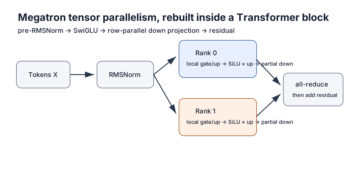
Megatron training is often introduced through launcher flags: tensor parallelism, pipeline parallelism, sequence parallelism, distributed optimizer, recomputation, and process groups. That is useful when operating the framework, but it is a poor way to learn what the framework is doing.

I wanted to understand one smaller question first:

How can two ranks reproduce the forward pass, backward pass, and parameter update of one dense Transformer feed-forward sublayer without either rank storing the full intermediate width?

So I rebuilt that path with ordinary PyTorch and two CPU processes. The block is not a complete Transformer. It contains the part under test: pre-RMSNorm, a fused gate/up projection, SwiGLU, a down projection, and a residual connection.

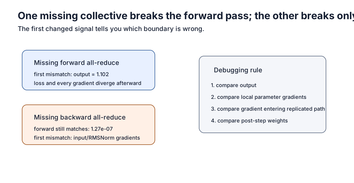
The finished two-rank step matched the dense reference to within 1.27e-07 in the forward pass and 1.49e-08 after one SGD update. More importantly, two deliberately broken versions failed in different places. Removing the forward reduction changed the output immediately. Removing the backward reduction left the output and loss correct, but corrupted the gradient entering RMSNorm.

That difference is the useful lesson. Tensor parallelism is not merely a way to divide weights. It is a way to divide one algebraic operation while restoring the missing sums at the exact boundaries where the dense computation requires them.

Start with the dense block

Here is the dense computation the two ranks must reproduce:

 1
 2
 3
 4
 5
 6
 7
 8
 9
10
11
12
13
14
15
16
17
18
19
20
21
22
23
24
25
26
27
28
29
30
31
32
33
34
35
36
37
38
39
40
41

class DenseSwiGLUBlock(nn.Module):
    r"""
                        ┌──────────────────────────────┐
                        │                              │
                        │        residual path         │
                        │                              ▼
    input x ────────────┼───────────────────────────── (+) ── output
                        │                              ▲
                        ▼                              │
                     RMSNorm                           │
                        │                              │
                 ┌──────┴──────┐                       │
                 ▼             ▼                       │
           gate projection   up projection             │
                 │             │                       │
                 ▼             │                       │
               SiLU            │                       │
                 │             │                       │
                 └────── × ────┘                       │
                        │                              │
                        ▼                              │
                 down projection ──────────────────────┘
    """

    def __init__(self, hidden_size: int, ffn_size: int):
        super().__init__()
        self.norm_weight = nn.Parameter(torch.ones(hidden_size))
        # Stack gate and up projections so the tensor-parallel version can shard the shared FFN dimension.
        self.w_gate_up = nn.Parameter(torch.empty(2, ffn_size, hidden_size))
        self.w_down = nn.Parameter(torch.empty(hidden_size, ffn_size))
        self.b_down = nn.Parameter(torch.zeros(hidden_size))

    def forward(self, x):
        residual = x
        x = rms_norm(x, self.norm_weight)

        gate = F.linear(x, self.w_gate_up[0])
        up = F.linear(x, self.w_gate_up[1])
        hidden = F.silu(gate) * up

        return residual + F.linear(hidden, self.w_down, self.b_down)

The executable fixture uses:

• sequence length S = 3;
• batch size B = 2;
• model width H = 8;
• feed-forward width F = 12;
• tensor-parallel size P = 2.

The dense shape trace is:

1
2
3
4
5
6
7

input                 [3, 2, 8]
RMSNorm output        [3, 2, 8]
gate projection       [3, 2, 12]
up projection         [3, 2, 12]
SwiGLU activation     [3, 2, 12]
down projection       [3, 2, 8]
residual output       [3, 2, 8]

The equations are:

The gate and up matrices each have shape [F, H]. The down matrix has shape [H, F]. That shared feed-forward dimension is the axis we will partition.

Split the expansion

The first change is to divide the gate and up projections by output feature. Each rank receives the full normalized token representation but computes only half of the feed-forward channels.

For two ranks:

Rank r computes:

The nonlinear operation remains local because each gate feature is paired with the corresponding up feature on the same rank.

1
2
3
4
5

normed_parallel = CopyToTensorParallelRegion.apply(normed)

gate_local = F.linear(normed_parallel, w_gate_up_local[0])
up_local = F.linear(normed_parallel, w_gate_up_local[1])
hidden_local = F.silu(gate_local) * up_local

Nothing needs to be summed in the forward pass yet. Rank 0 owns one set of feed-forward features; rank 1 owns the other. Concatenating those slices would recover the dense SwiGLU activation.

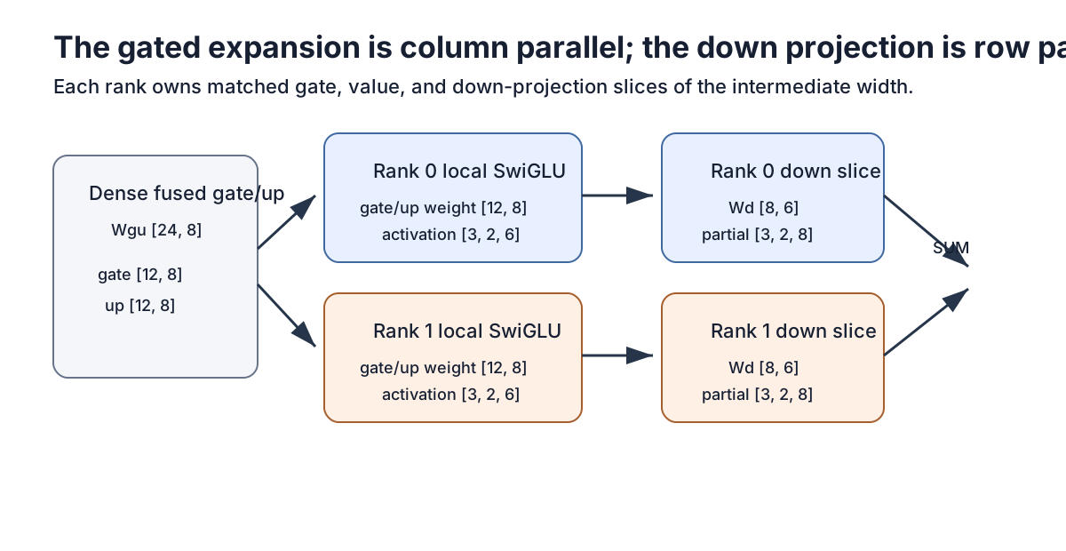
The shape correspondence is easier to see in one table:

In Megatron terminology, this expansion is the role played by a column-parallel linear layer: each rank owns different output columns of the logical projection.

Split the contraction

Now partition the down projection along its input feature dimension. Each rank consumes the SwiGLU slice it already owns:

Each rank computes a full-width but incomplete output:

The dense result is the sum of those partial products:

That equation tells us exactly where the first collective belongs.

1
2
3

partial = F.linear(hidden_local, w_down_local, None)
mlp_out = ReduceFromTensorParallelRegion.apply(partial)
out = residual + mlp_out + b_down

ReduceFromTensorParallelRegion performs an all-reduce in the forward pass:

 1
 2
 3
 4
 5
 6
 7
 8
 9
10

class ReduceFromTensorParallelRegion(torch.autograd.Function):
    @staticmethod
    def forward(ctx, x):
        y = x.clone()
        dist.all_reduce(y, op=dist.ReduceOp.SUM)
        return y

    @staticmethod
    def backward(ctx, grad_output):
        return grad_output

The backward pass through this operation is an identity. Every rank receives the same gradient for the replicated output, and each local down-projection shard uses that gradient to compute its own weight and activation gradients.

This is the row-parallel half of the pair: split the input features, compute partial outputs, and sum them.

Put the other collective in backward

The expansion layer has the opposite communication pattern.

Its forward pass needed no reduction because the output features were intentionally partitioned. But during backpropagation, every rank computes only the contribution from its local gate and up features to the gradient of the replicated normalized input.

For the dense input gradient:

That sum must happen before the gradient continues through RMSNorm and into the residual input. The custom operation around normed therefore does nothing in forward and reduces gradients in backward:

 1
 2
 3
 4
 5
 6
 7
 8
 9
10

class CopyToTensorParallelRegion(torch.autograd.Function):
    @staticmethod
    def forward(ctx, x):
        return x

    @staticmethod
    def backward(ctx, grad_output):
        grad = grad_output.clone()
        dist.all_reduce(grad, op=dist.ReduceOp.SUM)
        return grad

The two communication rules are now paired:

This maps to the core Megatron pattern:

The fixture implements these semantics directly with torch.distributed; it does not import Megatron-Core classes.

Reproduce one dense training step

First inspect the actual environment, block, and tensor shapes:

1
2

python -m torch.distributed.run --standalone --nproc_per_node=2 \
  code/megatron_tp_mlp.py --mode inspect

 1
 2
 3
 4
 5
 6
 7
 8
 9
10
11
12
13
14
15
16
17
18
19
20
21
22

{
  "python": "3.13.5",
  "pytorch": "2.10.0+cpu",
  "backend": "gloo",
  "world_size": 2,
  "block_path": "pre-RMSNorm -> fused gate/up -> SwiGLU -> down projection -> residual add",
  "dense_shapes": {
    "x": [3, 2, 8],
    "norm_weight": [8],
    "w_gate_up": [2, 12, 8],
    "w_down": [8, 12],
    "output": [3, 2, 8]
  },
  "rank_local_shapes": {
    "gate_up_weight": [2, 6, 8],
    "gate": [3, 2, 6],
    "up": [3, 2, 6],
    "swiglu": [3, 2, 6],
    "down_weight": [8, 6],
    "partial_output": [3, 2, 8]
  }
}

The launcher’s Gloo connection lines are omitted from this embedded excerpt; the complete retained output is in data/terminal-01-inspect.txt. The environment record is in data/environment.json.

Now compare one complete sharded training step with the dense reference initialized from the same tensors:

1
2

python -m torch.distributed.run --standalone --nproc_per_node=2 \
  code/megatron_tp_mlp.py --mode equivalence

 1
 2
 3
 4
 5
 6
 7
 8
 9
10
11
12
13

{
  "mode": "equivalence",
  "world_size": 2,
  "forward_max_abs_diff": 1.2665987014770508e-07,
  "loss_abs_diff": 0.0,
  "input_grad_max_abs_diff": 2.9802322387695312e-08,
  "norm_grad_max_abs_diff": 1.4901161193847656e-08,
  "gate_up_grad_max_abs_diff": 4.470348358154297e-08,
  "down_grad_max_abs_diff": 2.2351741790771484e-08,
  "down_bias_grad_max_abs_diff": 2.2351741790771484e-08,
  "post_step_weight_max_abs_diff": 1.4901161193847656e-08,
  "passed": true
}

The complete transcript is data/terminal-02-equivalence.txt.

The differences are consistent with floating-point operation ordering. Within this CPU fixture, the two-rank path reproduces the dense forward pass, backward pass, and parameter update.

Remove each collective

An equivalence result is useful only if the test can reject plausible wrong implementations. The two broken versions below are designed to fail at different points.

Remove the forward reduction

Prediction: each rank will treat a partial down-projection result as the complete MLP output, so the first mismatch should appear in the forward output.

1
2

python -m torch.distributed.run --standalone --nproc_per_node=2 \
  code/megatron_tp_mlp.py --mode missing_forward_reduce

 1
 2
 3
 4
 5
 6
 7
 8
 9
10
11
12

{
  "mode": "missing_forward_reduce",
  "world_size": 2,
  "forward_max_abs_diff": 1.1021764278411865,
  "loss_abs_diff": 0.19488954544067383,
  "input_grad_max_abs_diff": 0.03851410746574402,
  "norm_grad_max_abs_diff": 0.04135049879550934,
  "gate_up_grad_max_abs_diff": 0.05925934761762619,
  "down_grad_max_abs_diff": 0.026660695672035217,
  "post_step_weight_max_abs_diff": 0.0036689937114715576,
  "passed": false
}

The retained output is data/terminal-03-missing-forward.txt.

The prediction holds. The first changed signal is the model output, with a maximum error of 1.10. Once the loss is computed from the wrong output, every downstream gradient is also wrong.

Remove the backward reduction

Prediction: the forward output and loss will still match because the row-parallel forward sum remains intact. The first mismatch should appear only when gradients from the two local expansion shards need to be combined before RMSNorm.

1
2

python -m torch.distributed.run --standalone --nproc_per_node=2 \
  code/megatron_tp_mlp.py --mode missing_backward_reduce

 1
 2
 3
 4
 5
 6
 7
 8
 9
10
11
12

{
  "mode": "missing_backward_reduce",
  "world_size": 2,
  "forward_max_abs_diff": 1.2665987014770508e-07,
  "loss_abs_diff": 0.0,
  "input_grad_max_abs_diff": 0.13864503800868988,
  "norm_grad_max_abs_diff": 0.20240136981010437,
  "gate_up_grad_max_abs_diff": 4.470348358154297e-08,
  "down_grad_max_abs_diff": 2.2351741790771484e-08,
  "post_step_weight_max_abs_diff": 0.010120153427124023,
  "passed": false
}

The retained output is data/terminal-04-missing-backward.txt.

This is the more revealing failure. The forward output still agrees to 1.27e-07, and the loss is identical. The local gate/up and down-projection gradients also match. Yet the input gradient differs by 0.139, the RMSNorm-weight gradient differs by 0.202, and one optimizer step moves the parameters apart by 0.0101.

A forward-only test would approve this broken training graph.

The distributed test suite checks all four cases:

1

pytest -q code/test_megatron_tp_mlp.py

1
2

....                                                                     [100%]
4 passed in 26.94s

The retained test output is data/terminal-05-tests.txt. The complete implementation is code/megatron_tp_mlp.py, and the direct tests are code/test_megatron_tp_mlp.py.

What this reconstruction proves—and what it does not

The small implementation establishes one precise result: for this pre-RMSNorm SwiGLU feed-forward block, partitioning the expansion by output features and the contraction by input features reproduces dense training when the partial contraction outputs are summed in forward and the partial replicated-input gradients are summed in backward.

It also shows why the two reductions need separate tests. A missing forward collective is visible immediately. A missing backward collective can survive output and loss checks while silently corrupting upstream learning.

The fixture does not execute Megatron-Core. It does not test:

• self-attention or a complete Transformer block;
• sequence parallelism;
• CUDA or NCCL collective behavior;
• BF16 or FP8 arithmetic;
• fused RMSNorm, SwiGLU, or linear kernels;
• asynchronous communication overlap;
• gradient accumulation;
• pipeline parallelism;
• distributed optimizer state;
• more than two tensor-parallel ranks.

Those are not cosmetic differences. For example, sequence parallelism changes which activations are replicated, fused kernels change numerical ordering, and larger process groups change communication cost and failure behavior.

Still, the reconstruction changes how I read Megatron code. I no longer start with “which tensors are split?” I start with the dense equation and ask two questions:

1. Which sum has been replaced by independent local products?
2. At what point must those products be combined so forward and backward remain equivalent?

For the feed-forward block, those questions lead directly to the matched column-parallel and row-parallel projections—and to one collective in each direction.

References

• NVIDIA, Megatron Core User Guide.
• NVIDIA, Megatron Core parallelism strategies.
• NVIDIA, Tensor-parallel layers API.