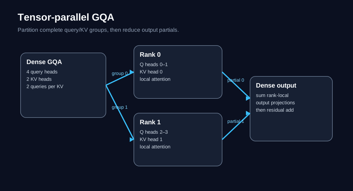
Grouped-query attention creates a partitioning problem that ordinary multi-head attention can hide. There are more query heads than key/value heads, so several query heads reuse the same KV head. If a tensor-parallel split cuts projection matrices at an arbitrary width, it can separate a query head from the KV head it is supposed to share.

I wanted to reconstruct the smallest attention block that still preserves that constraint. The reference is a pre-RMSNorm, causal GQA layer with rotary position embeddings, four query heads, two KV heads, and a residual connection. I then turn it into two rank-local attention paths in visible steps and compare the resulting training update against the dense block.

The result is narrow but useful: the natural partition is a complete query/KV group, not an arbitrary matrix slice. The forward pass also needs an output reduction, while the replicated input path needs a separate backward reduction. A forward-only test catches the first bug and misses the second.

Start with the dense block

The dense reference is short enough to inspect:

 1
 2
 3
 4
 5
 6
 7
 8
 9
10
11
12
13
14
15
16
17
18
19
20
21
22
23
24
25
26
27
28
29
30
31
32
33
34
35
36
37
38

def apply_rope(x):
    """
    x[..., :half] ─┐
                   ├─ rotate by position/frequency phase ── RoPE(x)
    x[..., half:] ─┘
    """
    # x: [S,B,H,D], D even
    s = x.shape[0]
    half = x.shape[-1] // 2
    pos = torch.arange(s, dtype=x.dtype, device=x.device).view(s,1,1,1)
    freq = torch.arange(half, dtype=x.dtype, device=x.device).view(1,1,1,half)
    theta = pos / (10000.0 ** (freq / max(1, half)))
    c, si = theta.cos(), theta.sin()
    a, b = x[..., :half], x[..., half:]
    return torch.cat([a*c - b*si, a*si + b*c], dim=-1)


def repeat_kv(x, groups):
    """
    KV heads [S,B,Hkv,D] ── repeat each head `groups` times ── [S,B,Hq,D]
    """
    return x.repeat_interleave(groups, dim=2)


def dense_forward(x, p, cfg):
    """
    x ── RMSNorm ── Q,K,V ── RoPE ── repeat KV ── attention ── output proj ─┐
    └──────────────────────────────────────── residual ─────────────────── (+)
    """
    residual = x
    n = rms_norm(x, p['norm'], cfg.eps)
    q = F.linear(n, p['wq']).view(cfg.seq,cfg.batch,cfg.query_heads,cfg.head_dim)
    k = F.linear(n, p['wk']).view(cfg.seq,cfg.batch,cfg.kv_heads,cfg.head_dim)
    v = F.linear(n, p['wv']).view(cfg.seq,cfg.batch,cfg.kv_heads,cfg.head_dim)
    q, k = apply_rope(q), apply_rope(k)
    groups = cfg.query_heads // cfg.kv_heads
    ctx = attention(q, repeat_kv(k, groups), repeat_kv(v, groups))
    return residual + F.linear(ctx.reshape(cfg.seq,cfg.batch,-1), p['wo'])

The model dimensions are intentionally tiny, but the semantic axes are real:

The first terminal command records the actual fixture and versions:

1

PYTHONPATH=code python code/tp_gqa_attention.py --mode inspect

 1
 2
 3
 4
 5
 6
 7
 8
 9
10
11
12
13
14
15
16
17
18
19
20
21
22
23
24

{
  "python": "3.13.5",
  "pytorch": "2.10.0+cpu",
  "config": {
    "seq": 5,
    "batch": 2,
    "hidden": 16,
    "query_heads": 4,
    "kv_heads": 2,
    "head_dim": 4,
    "world_size": 2,
    "eps": 1e-06
  },
  "dense_shapes": {
    "x": [5, 2, 16],
    "q": [5, 2, 4, 4],
    "k_v": [5, 2, 2, 4]
  },
  "rank_local": {
    "query_heads": 2,
    "kv_heads": 1
  },
  "rule": "keep complete query/KV groups on each rank; sum output-projection partials"
}

The full transcript is retained in data/terminal-01-inspect.txt, and the executable reference is in code/tp_gqa_attention.py.

First change: split complete head groups

Each KV head is shared by exactly two query heads. That gives two indivisible groups:

1
2

group 0: query heads 0, 1  +  KV head 0
group 1: query heads 2, 3  +  KV head 1

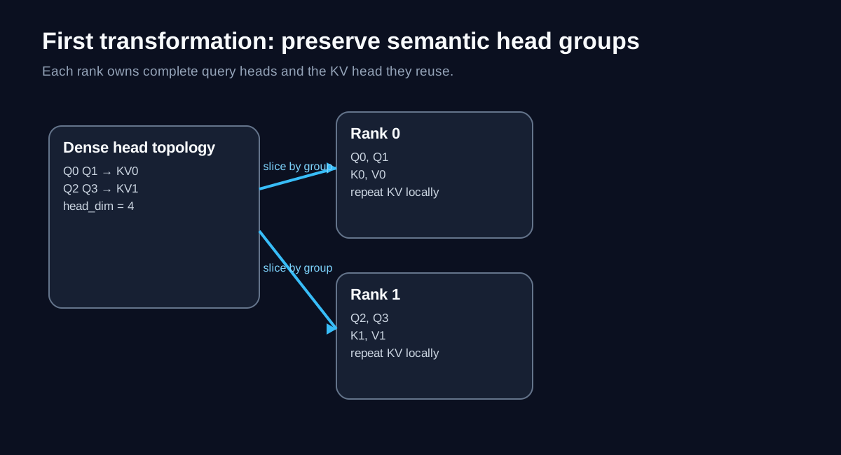
Rank 0 receives group 0. Rank 1 receives group 1. In matrix terms, the Q projection is split by blocks of 2 × head_dim = 8 output rows, while K and V are split by blocks of 1 × head_dim = 4 output rows.

The local code is the dense code with smaller head counts:

 1
 2
 3
 4
 5
 6
 7
 8
 9
10

q_local = F.linear(n, wq_local).view(S, B, 2, 4)
k_local = F.linear(n, wk_local).view(S, B, 1, 4)
v_local = F.linear(n, wv_local).view(S, B, 1, 4)

q_local = apply_rope(q_local)
k_local = apply_rope(k_local)

k_local = repeat_kv(k_local, groups=2)
v_local = repeat_kv(v_local, groups=2)
context_local = causal_attention(q_local, k_local, v_local)

No communication is needed inside this local attention calculation. RoPE operates within each head, the causal mask is shared, and the rank already owns the KV head needed by both of its query heads. This matches the original Megatron observation that attention heads can be computed locally after Q, K, and V are column-partitioned by head ownership.

The important restriction is divisibility. With two TP ranks, two KV heads divide cleanly. A configuration with two KV heads and four TP ranks cannot assign one complete KV head to every rank without replication or a different layout. The toy fixture does not solve that more general case.

Second change: split the output projection

Local attention produces only half of the dense context width:

The dense output projection has shape [hidden, query_heads × head_dim] = [16, 16]. Each rank owns the columns corresponding to its local context features. If C^(r) is rank r’s local context and W_o^(r) is the matching column slice, then

Each rank can compute a full-width partial:

1
2
3
4

partial = F.linear(
    context_local.reshape(S, B, -1),
    wo_local,
)

But no partial is the dense answer. The rank-local outputs must be summed before the residual addition.

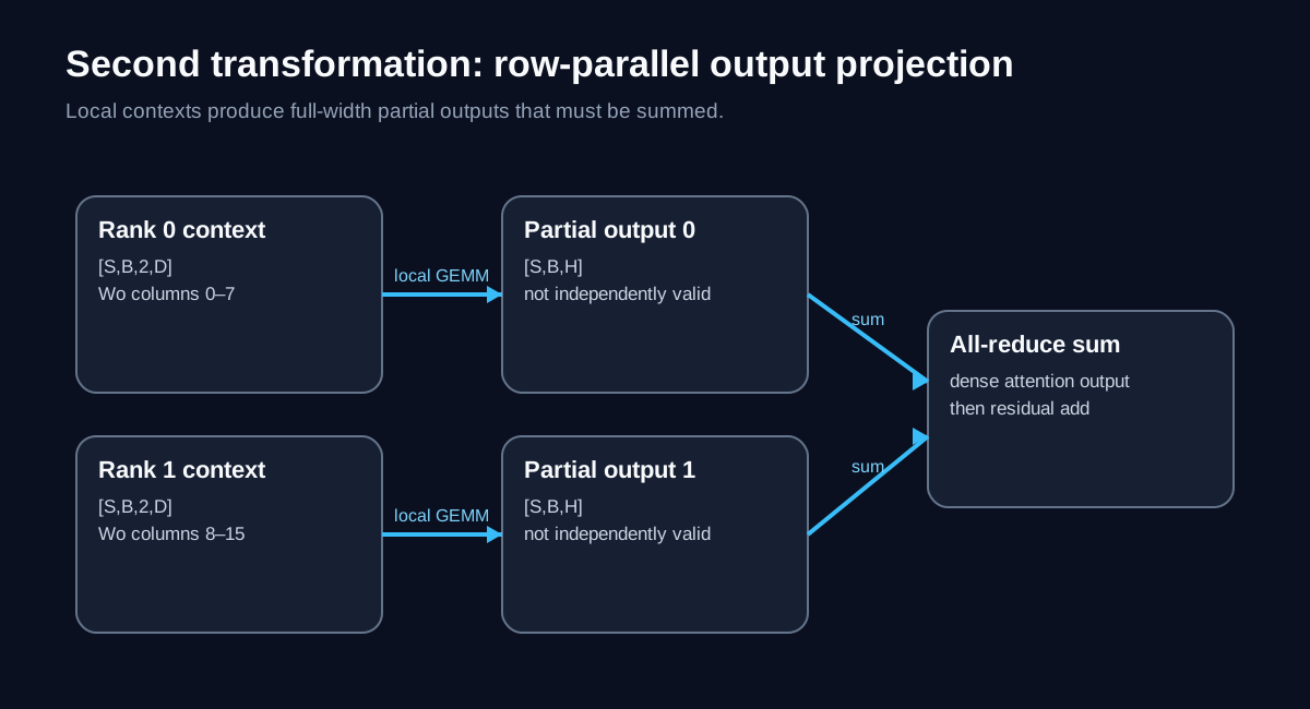
This is the row-parallel half of the reconstruction. It also explains why gathering the local contexts first would be wasteful: the output projection can consume the partitioned context directly, and only its full-width partial outputs need to be reduced.

Rebuild the complete training step

The compact tensor-parallel path now has two transformations:

1. partition Q, K, and V by complete GQA head groups;
2. partition the output projection by the corresponding context features and sum the partial outputs.

The implementation uses one process to make the algebra easy to inspect, while treating the two branches as rank-local computations with shared parameters sliced exactly as two TP ranks would own them. It is therefore a numerical reconstruction of the TP layer, not a benchmark of distributed communication.

Run the direct comparison:

1

PYTHONPATH=code python code/tp_gqa_attention.py --mode equivalence --seed 11

 1
 2
 3
 4
 5
 6
 7
 8
 9
10

{
  "seed": 11,
  "mode": "equivalence",
  "forward_max_abs_diff": 1.1920928955078125e-07,
  "loss_abs_diff": 0.0,
  "input_grad_max_abs_diff": 3.725290298461914e-09,
  "parameter_grad_max_abs_diff": 2.2351741790771484e-08,
  "post_step_weight_max_abs_diff": 1.4901161193847656e-08,
  "passed": true
}

The comparison uses identical inputs, parameters, target tensor, MSE loss, and SGD learning rate. It checks more than the visible output:

Those residuals are consistent with different floating-point accumulation order, not a different computation. The retained five-seed results are in data/results.csv and data/results.json.

Break forward and backward separately

A reconstruction is more convincing when a plausible wrong version fails for the reason predicted by the algebra.

Remove the output reduction

Prediction: the first wrong signal should be the forward output because one rank-local partial is being mistaken for the complete output.

1
2

PYTHONPATH=code python code/tp_gqa_attention.py \
  --mode missing_output_reduce --seed 11

 1
 2
 3
 4
 5
 6
 7
 8
 9
10

{
  "seed": 11,
  "mode": "missing_output_reduce",
  "forward_max_abs_diff": 0.700843870639801,
  "loss_abs_diff": 0.05957293510437012,
  "input_grad_max_abs_diff": 0.013707960024476051,
  "parameter_grad_max_abs_diff": 0.12953613698482513,
  "post_step_weight_max_abs_diff": 0.0064768195152282715,
  "passed": false
}

The prediction holds. Across five seeds, the forward error ranges from 0.324 to 0.937. Everything downstream is already operating on the wrong activation.

Remove the replicated-input gradient reduction

The less obvious bug is in backward. Both column-partitioned projection branches read the same normalized input. In a real TP implementation, each rank computes only its local contribution to the gradient with respect to that replicated input. Those contributions must be summed.

The fixture simulates a missing reduction by allowing both branches to contribute in forward while dropping rank 1’s contribution to the upstream input gradient.

Prediction: the forward output and loss should still match, but the first wrong signal should be dX.

1
2

PYTHONPATH=code python code/tp_gqa_attention.py \
  --mode missing_input_grad_reduce --seed 11

 1
 2
 3
 4
 5
 6
 7
 8
 9
10

{
  "seed": 11,
  "mode": "missing_input_grad_reduce",
  "forward_max_abs_diff": 1.1920928955078125e-07,
  "loss_abs_diff": 0.0,
  "input_grad_max_abs_diff": 0.01103300042450428,
  "parameter_grad_max_abs_diff": 0.0307764932513237,
  "post_step_weight_max_abs_diff": 0.0015388727188110352,
  "passed": false
}

The forward check passes within the same tolerance as the correct implementation. Training is still wrong. Across five seeds, the input-gradient error ranges from 0.00998 to 0.0182.

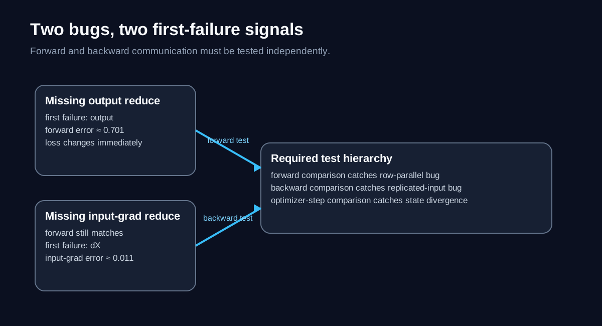
The test hierarchy now follows directly from the mechanism:

• compare forward outputs to catch a missing row-parallel output reduction;
• compare input and parameter gradients to catch missing backward communication;
• compare updated parameters to confirm that the entire state transition matches.

Run the suite:

1

PYTHONPATH=code pytest -q code/test_tp_gqa_attention.py

1
2

.....                                                                    [100%]
5 passed in 9.92s

The full test output is retained in data/terminal-05-tests.txt.

How this maps to Megatron Core

The reconstruction is deliberately written with ordinary PyTorch functions, but the objects map cleanly to Megatron’s tensor-parallel design:

The original Megatron-LM design partitions Q, K, and V so complete attention heads stay local, then row-partitions the output projection. NVIDIA’s current Megatron Core documentation still describes tensor parallelism as splitting individual layers, while the production implementation adds sequence parallelism, process-group management, communication overlap, Transformer Engine kernels, and hardware-specific collectives.

This post does not establish performance, communication cost, or correctness for Megatron Core itself. It does not run CUDA, NCCL, FlashAttention, sequence parallelism, context parallelism, mixed precision, fused QKV layouts, KV replication for awkward GQA ratios, dropout RNG tracking, or distributed optimizer state. Those are the next layers of the reconstruction.

What the reconstruction made visible

I started with the intuition that tensor parallelism partitions projection matrices. That is mechanically true but not precise enough for GQA. The reusable rule is semantic: keep each query/KV reuse group intact, let attention remain local, and place reductions at the boundaries where independently computed contributions must become one tensor.

The forward reduction and backward reduction are separate obligations. The second one is easy to miss because the model can produce the correct output while training with the wrong gradient. After this reconstruction, I would not approve a tensor-parallel attention change from forward parity alone.

References

• Joshua Ainslie et al., “GQA: Training Generalized Multi-Query Transformer Models from Multi-Head Checkpoints”, 2023.
• Mohammad Shoeybi et al., “Megatron-LM: Training Multi-Billion Parameter Language Models Using Model Parallelism”, 2019.
• NVIDIA, Megatron Core parallelism strategies.
• NVIDIA, Megatron-LM source repository.