What are the priorities of distributed training?
Let’s get this straight to start with - distributed training is first and foremost about jumping over the Memory Wall, less about speed.
A single expensive H100 GPU has 80GB of memory, which to poor old engineers like me who remember the joy of getting their hands on 48GB GPUs seems like a dream, but a 70B parameter model requires around 140GB just to store the weights in 16-bit precision, not counting the optimizer states (which take significantly more space) or activation memory.
So the primary goal of setting up training is to architect a system to fit a massive data transform/equation across a cluster of hardware without letting the communication overhead kill your throughput.
This has two dimensions - from research of ML scientists and mathematicians, we regularly receive clever architecture optimizations that enhance the performance and efficiency of models. Secondly, from the understanding the implementations of these models and testing by ML engineers, we have made a lot of hardware aligned improvements to how models are trained and served.
3D Parallelism

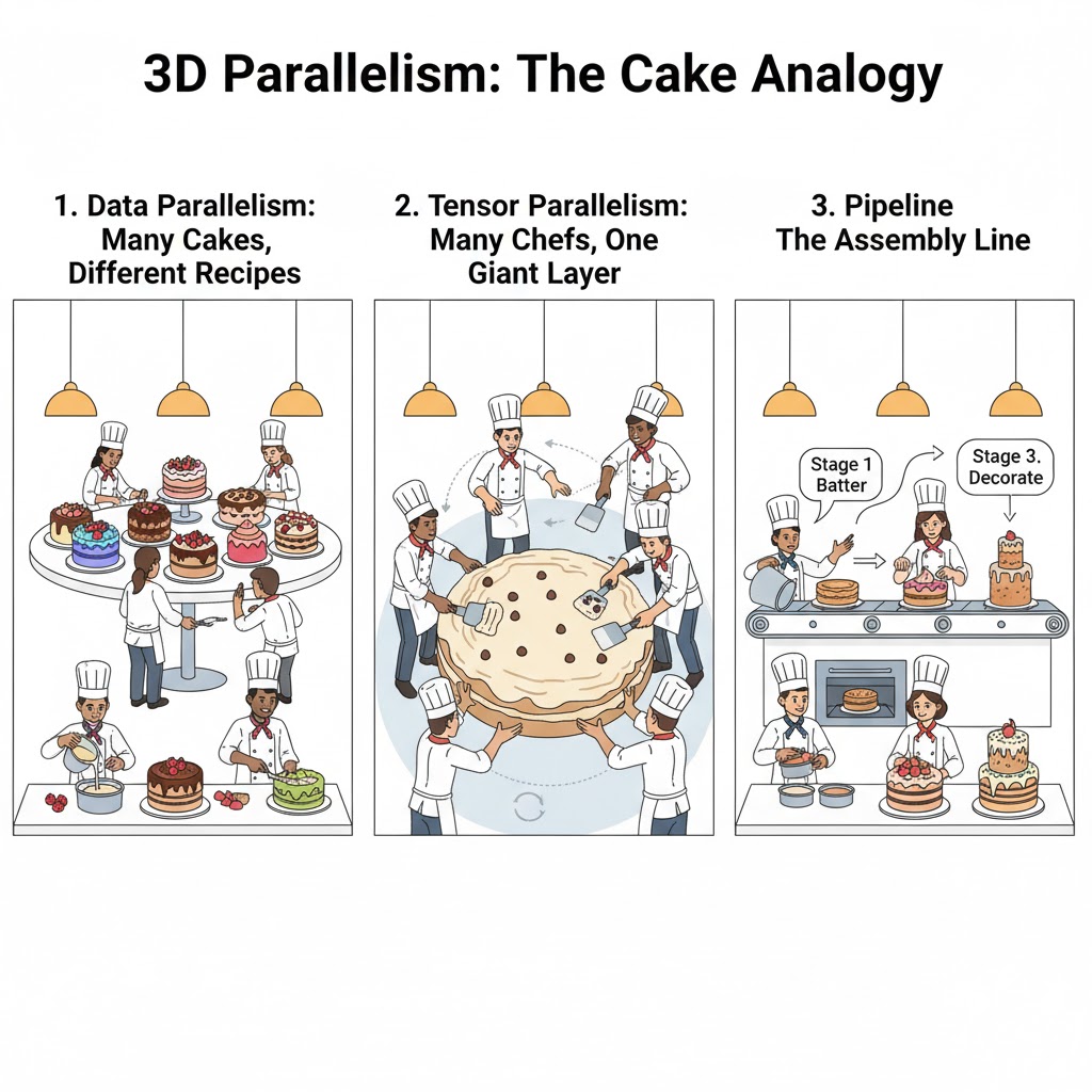
Alright, so let’s assume we are learning to bake a cake with 10 chefs (GPUs).
- Data Parallelism: In this case, input data gets sliced. Each of the 10 chefs bakes a whole separate cake, each using different ingredients (data) in parallel.
- Tensor Parallelism: In this case, the model matrices in each layer get sliced. 10 chefs working on the same cake layer at the exact same time (one mixes, one pours etc.).
- Pipeline Parallelism: In this case, the layers in terms of model depth get sliced. An assembly line: Chef 1 makes the batter, Chef 2 bakes, Chef 3 frosts.
It is a balancing act to make decisions on which approach to favor for each use case - training, inference etc. A short guide to help focus on an aspect of parallelism:
| Dimension | Communication Style | Key Benefit (Pro) | Key Bottleneck (Con) |
|---|---|---|---|
| Data Parallelism | All-Reduce (Syncs gradients at end) | Easiest to implement; scales throughput linearly. | VRAM: Every GPU stores a full copy of the model. |
| Tensor Parallelism | All-Gather (Syncs constantly) | Reduces memory usage for massive layers. | Bandwidth: Needs ultra-fast cables (NVLink) or it slows down. |
| Pipeline Parallelism | Point-to-Point (Passes baton) | Allows models larger than single-GPU memory. | Idle Time: GPUs wait around for data. |
Shout out to this video for more in depth details!
Tech Stack
Often related to the size of the models to be trained, we can make decisions to use certain tools.
1. The “start here” tools:
Pytorch Data Parallel (DP): Only works on a single node because it uses single process, multiple threads. How it works is the main GPU, called the driver, holds the model and data. For every batch, it scatters data to other GPUs → then replicates the model to them → runs the forward pass → gathers the outputs → computes the loss → then scatters the calculated gradients. If you are familiar with how python multiprocessing works, this means that the Global Interpreter Lock (GIL) comes into play. Only one of the threads can hold the GIL at a time, so the others have to wait their turn (zzzzzs). Additionally, the main GPU (#0) has heavy memory pressure because along with holding its own weights and data, it also has to gather the output tensors sent by other GPUs to calculate the loss (All gather approach).
Distributed Data Parallel (DDP): As you can tell, this approach improves DP by using multiple processes. Every GPU runs its own independent Python process. They all load the model once at the start. They only communicate to sync gradients (All reduce approach) at the very end of a backward pass. Another advantage of this is that it can work on multiple nodes due to network backends like NCCL or Gloo. The bottleneck here is that they are independent process and don’t know what the other processes are up to. So they need to find a way to tell the other processes “I’m done!” - this usually happens by posting to a master address and port to sync with other processes and proceed to the next step.
2. Memory Sharding: “redundancy elimination” tools
In standard Distributed Data Parallel (DDP), if you have 4 GPUs, you store 4 identical copies of the model, 4 identical copies of the optimizer states, and 4 identical copies of the gradients. That is a massive waste of precious VRAM - so what can we do? We can shard/slice everything.
Instead of every GPU holding the full picture, each GPU holds only a fraction of the data and weights. When a GPU needs a specific weight to do a calculation, it quickly asks its neighbors for it, uses it, and then discards it.
This is a very suitable approach to train 7B-70B models without applying complex 3D parallelism. It should be the next stage in optimizing your pipeline after DDP.
DeepSpeed ZeRO
There are 3 stages that correspond to how much we want to shard.
Stage 1: Optimizer Sharding
Optimizer states are probably the biggest memory hogs while training, and only sharding the optimizer states (like momentum in Adam) can reduce memory usage significantly. The model weights and data are still fully replicated across the GPUs.
Stage 2: Gradient Sharding
Now we shard the optimizer state and gradient calculated for each parameter. Adds more memory saving with very little communication overhead. Probably worth doing in most scenarios.
Stage 3: Parameter/Weight Sharding
Now the weights join the party. No GPU now holds any part of the model, optimizer or gradients. Now you can start fitting models larger than the VRAM of a single GPU itself.
PyTorch FSDP (Fully Sharded Data Parallel)
This is basically PyTorch native implementation of ZeRO Stage 3.
3. Heavy lifters: Tensor Parallelism (TP) through Megatron-LM
Good for training >70B parameter models
While sharding slices the data or the storage of weights, Megatron-LM slices the math itself. When a weight matrix cannot fit in a single GPU, we can slice it across GPUs. However, we need to do this in a manner where each GPU can work on a chunk of the matrix independently before they need to communicate.
Let’s consider a simple MLP/feedforward layer’s matrix multiplication. Let’s say it consists of 2 matrices A and B and an input X, and you have 2 GPUs.
- Column Parallel: Slice matrix A by columns, and spread the multiplication of X with each slice of A. GPU 0 calculates the “left half” of the output vectors; GPU 1 calculates the “right half.”
- Row Parallel: Now to multiply the outputs of column parallel without needing to sync up yet—slice B by row/horizontally. Because GPU 0 is holding the “left half” of the data, we give it the “top half” of matrix B (which corresponds to those left-side features). At the end of this operation, we have partial columns of A multiplied by partial rows of B.
- The Sync: Now, finally we can apply an All-Reduce that sums up the outputs of each GPU to generate the final result.